Logistic and Bayesian Binomial Models - Modeling SSI Risk After Colon Surgery in California

library(arrow)
library(rjags)

# Load data
colon_fac_ach <- read_parquet("data/colon_fac_ach.parquet")

Warning message:
“package ‘arrow’ was built under R version 4.5.2”

Attaching package: ‘arrow’


The following object is masked from ‘package:utils’:

    timestamp


Loading required package: coda

Linked to JAGS 4.3.2

Loaded modules: basemod,bugs

Binomial logistic regression¶

Below, a standard logistic regression model is fit to the data. Community, <125 Beds facilities are used for the reference group.


Call:
glm(formula = cbind(Infections_Reported, No_Infections) ~ Facility_Type, 
    family = binomial, data = colon_fac_ach)

Coefficients:
                                     Estimate Std. Error z value Pr(>|z|)    
(Intercept)                           -4.3979     0.2012 -21.856  < 2e-16 ***
Facility_TypeCommunity, >250 Beds      0.6069     0.2194   2.767  0.00566 ** 
Facility_TypeCommunity, 125-250 Beds   0.4526     0.2326   1.946  0.05165 .  
Facility_TypeMajor Teaching            0.6122     0.2076   2.949  0.00318 ** 
---
Signif. codes:  0 ‘***’ 0.001 ‘**’ 0.01 ‘*’ 0.05 ‘.’ 0.1 ‘ ’ 1

(Dispersion parameter for binomial family taken to be 1)

    Null deviance: 495.24  on 287  degrees of freedom
Residual deviance: 483.68  on 284  degrees of freedom
AIC: 977.75

Number of Fisher Scoring iterations: 5

The standard logistic regression with facility type as the only factor with 4 levels produces only 4 predicted probabilities, which does not adequately explain the large variation observed across individual facilities. This model treats all facilities of the same type identically, ignoring facility volume and county-level effects.

Bayesian binomial model¶

The Bayesian binomial model is fit next. Weakly informative $\text{N}(0, 5^2)$ priors are used for the parameters.

\begin{aligned} y_i \mid \phi_i &\sim \text{Binomial}(n_i, \phi_i), \quad i = 1, \dots, 288 \\ \text{logit}(\phi_i) &= \beta_0 + \beta_1 \cdot \text{beds}_{125\text{-}250,i} + \beta_2 \cdot \text{beds}_{>250,i} + \beta_3 \cdot \text{major\_teach}_i \\ \beta_k &\sim \text{Normal}(0, 5^2), \quad k = 0,1,2,3 \end{aligned}

(1)

JAGS model syntax¶

## Non-hierarchical Bayesian binomial model

# Transform data for JAGS; use Community, <125 Beds for reference level
data_jags_nh <- list(
  y = colon_fac_ach$Infections_Reported,
  n = colon_fac_ach$Procedure_Count,
  beds_125to250 = 
    as.numeric(colon_fac_ach$Facility_Type == 'Community, 125-250 Beds'),
  beds_gt250 = 
    as.numeric(colon_fac_ach$Facility_Type == 'Community, >250 Beds'),
  major_teach = as.numeric(colon_fac_ach$Facility_Type == 'Major Teaching'),
  N = nrow(colon_fac_ach),
  J = 3  # number of predictors
)

# Model syntax
mod_string_nh <- " model {
  # likelihood
  for (i in 1:N) {
    y[i] ~ dbin(p[i], n[i])
    logit(p[i]) <- b0 + b[1]*beds_125to250[i] + b[2]*beds_gt250[i] + 
                        b[3]*major_teach[i]
  }

  # priors
  b0 ~ dnorm(0, 1.0/5^2)
  for (j in 1:J) {
    b[j] ~ dnorm(0.0, 1.0/5^2)  # weakly informative priors (sd ~5)
  }
} "

# Model setup
set.seed(530)

# Define seeds for JAGS chains
jags_seeds <- list(
  list(.RNG.name = "base::Wichmann-Hill", .RNG.seed = 530),
  list(.RNG.name = "base::Wichmann-Hill", .RNG.seed = 531),
  list(.RNG.name = "base::Wichmann-Hill", .RNG.seed = 532)
)

mod_nh <- jags.model(textConnection(mod_string_nh),
                     data = data_jags_nh,
                     inits = jags_seeds,
                     n.chains = 3)

update(mod_nh, 1e4)  # burn-in

params_nh <- c("b0", "b")

# Run model
mod_sim_nh <- coda.samples(mod_nh, variable.names = params_nh, n.iter = 1e5)

Compiling model graph
   Resolving undeclared variables
   Allocating nodes
Graph information:
   Observed stochastic nodes: 288
   Unobserved stochastic nodes: 4
   Total graph size: 1466

Initializing model

Diagnostics¶

Trace plots¶

plot(mod_sim_nh)

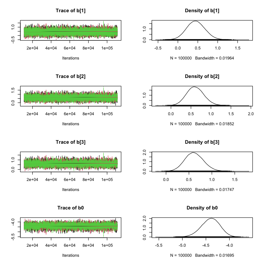
The chains exhibit autocorrelation, particularly for the intercept, but show good mixing around a stable posterior mean, with no evidence of non-convergence.

Autocorrelation¶

An autocorrelation table and plots for the second chain are shown below.

# Autocorrelation table and plots
autocorr.diag(mod_sim_nh)

autocorr.plot(mod_sim_nh[[2]], lag.max = 175)

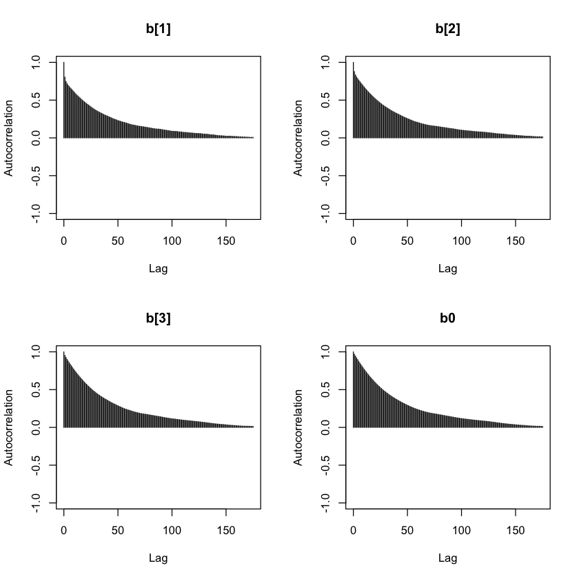
The MCMC chains exhibit high autocorrelation at short lags (lag-1 correlations 0.80–0.97), which gradually decreases at longer lags (lag-50 correlations 0.22–0.28), with good mixing achieved after approximately 150–200 iterations.

Gelman-Rubin¶

The Gelman-Rubin convergence diagnostic is shown below.

gelman.diag(mod_sim_nh)

Potential scale reduction factors:

     Point est. Upper C.I.
b[1]          1       1.00
b[2]          1       1.01
b[3]          1       1.01
b0            1       1.01

Multivariate psrf

1

Convergence diagnostics indicated good mixing across chains. All Gelman-Rubin PSRF values are equal to 1 (both univariate and multivariate), suggesting that between-chain and within-chain variances were indistinguishable and that the MCMC chains had converged to a common posterior distribution.

Effective sample sizes¶

Effective sample sizes are shown below.

round(effectiveSize(mod_sim_nh), 1)

Despite high autocorrelation in the MCMC chains, the effective sample sizes for all parameters are high, indicating that the posterior estimates are based on several thousand independent-equivalent draws. This provides confidence in the accuracy and stability of the posterior summaries.

Raftery-Lewis diagnostics¶

Raftery-Lewis diagnostics for the second chain are shown below.

raftery.diag(mod_sim_nh[[2]])


Quantile (q) = 0.025
Accuracy (r) = +/- 0.005
Probability (s) = 0.95 
                                             
      Burn-in  Total  Lower bound  Dependence
      (M)      (N)    (Nmin)       factor (I)
 b[1] 65       65871  3746         17.6      
 b[2] 78       81601  3746         21.8      
 b[3] 84       95496  3746         25.5      
 b0   100      106720 3746         28.5

Raftery-Lewis diagnostics indicate that the MCMC chains are moderately autocorrelated, particularly for the intercept (b0), with dependence factors up to 29. Recommended total iterations to estimate the 0.025 quantile to ±0.005 accuracy are 65,000–110,000 depending on the parameter. Given that 90,000 iterations were run after burn-in, the chains provide sufficient information for posterior summaries, although extreme quantiles of the intercept may be slightly less precise.

Deviance information criterion (DIC)¶

The DIC statistic for the model is shown below.

(dic_nh <- dic.samples(mod_nh, n.iter = 1e3))

Mean deviance:  973.9 
penalty 4.364 
Penalized deviance: 978.3

For the current Bayesian binomial model, the mean deviance is 973.9 with a small effective number of parameters (4.36), resulting in a penalized deviance (DIC) of 978.3. This serves as a baseline for comparison with more complex models, such as the hierarchical model.

Model summary¶

The results of the fitted model are shown below.

summary(mod_sim_nh)


Iterations = 11001:111000
Thinning interval = 1 
Number of chains = 3 
Sample size per chain = 1e+05 

1. Empirical mean and standard deviation for each variable,
   plus standard error of the mean:

        Mean     SD  Naive SE Time-series SE
b[1]  0.4508 0.2308 0.0004214       0.003227
b[2]  0.6079 0.2176 0.0003974       0.003244
b[3]  0.6157 0.2053 0.0003749       0.003247
b0   -4.4027 0.1993 0.0003638       0.003197

2. Quantiles for each variable:

         2.5%     25%     50%     75%  97.5%
b[1]  0.01073  0.2933  0.4462  0.6031  0.916
b[2]  0.19739  0.4588  0.6020  0.7512  1.050
b[3]  0.23016  0.4746  0.6091  0.7509  1.034
b0   -4.81178 -4.5330 -4.3958 -4.2655 -4.031

Compared with the reference group, all three groups have higher estimated probabilities of the outcome. On the log-odds scale, the posterior means are 0.45, 0.61, and 0.62 for groups 1–3, with 95% credible intervals largely above zero, suggesting that all groups are likely to differ from the reference group. These results are closely aligned with the binomial logistic regression results.