GLMM and Hierarchical Bayesian Models - Modeling SSI Risk After Colon Surgery in California

library(arrow)
library(lme4)
library(rjags)
library(kableExtra)
library(IRdisplay)
library(ggplot2)

# Load data
colon_fac_ach <- read_parquet("data/colon_fac_ach.parquet")

Warning message:
“package ‘arrow’ was built under R version 4.5.2”

Attaching package: ‘arrow’


The following object is masked from ‘package:utils’:

    timestamp


Loading required package: Matrix

Loading required package: coda

Linked to JAGS 4.3.2

Loaded modules: basemod,bugs

Random-intercepts GLMM¶

Facilities are nested within counties, creating a hierarchical data structure in which outcomes from facilities in the same county may be correlated due to shared local factors such as patient populations, referral patterns, or reporting practices.

To account for this clustering, a binomial generalized linear mixed model (GLMM) with a random intercept for county and fixed effects for facility type can be fit to the data. This specification allows the baseline log-odds of infection to vary across counties while estimating the average effect of facility type across all counties.

Each county $j$ is assigned a random intercept $u_j$ that represents its deviation from the overall mean log-odds. The model can be written as:

\text{logit}(p_{ij}) = \beta_0 + \beta_1 \text{FacilityType}_{ij} + u_j

(1)

where

$p_{ij}$ is the probability of SSI for facility $i$ in county $j$
$\beta_0$ is the overall intercept
$\beta_1$ is the fixed effect of facility type
$u_j \sim N(0, \sigma^2_\text{county})$ is the county-level random intercept

The following R code fits this GLMM to the observed data and displays the results.

Generalized linear mixed model fit by maximum likelihood (Laplace
  Approximation) [glmerMod]
 Family: binomial  ( logit )
Formula: cbind(Infections_Reported, No_Infections) ~ Facility_Type + (1 |  
    County)
   Data: colon_fac_ach

      AIC       BIC    logLik -2*log(L)  df.resid 
    943.3     961.6    -466.6     933.3       283 

Scaled residuals: 
    Min      1Q  Median      3Q     Max 
-2.0170 -0.7076 -0.3761  0.3658  6.6185 

Random effects:
 Groups Name        Variance Std.Dev.
 County (Intercept) 0.1779   0.4218  
Number of obs: 288, groups:  County, 42

Fixed effects:
                                     Estimate Std. Error z value Pr(>|z|)    
(Intercept)                           -4.4636     0.2175 -20.523  < 2e-16 ***
Facility_TypeCommunity, >250 Beds      0.6328     0.2283   2.772  0.00556 ** 
Facility_TypeCommunity, 125-250 Beds   0.3296     0.2373   1.389  0.16478    
Facility_TypeMajor Teaching            0.6146     0.2152   2.855  0.00430 ** 
---
Signif. codes:  0 ‘***’ 0.001 ‘**’ 0.01 ‘*’ 0.05 ‘.’ 0.1 ‘ ’ 1

Correlation of Fixed Effects:
            (Intr) F_TC>B F_TC1B
Fc_TC,>250B -0.834              
F_TC,125-2B -0.786  0.783       
Fclty_TypMT -0.882  0.887  0.829

The random-intercepts GLMM yields results that are broadly consistent with those from the standard logistic regression and Bayesian binomial models. Facilities classified as community hospitals with more than 250 beds and major teaching hospitals exhibit significantly higher odds of surgical site infection relative to the reference group, while the effect for community hospitals with 125 to 250 beds is positive but not statistically significant.

The estimated county-level random intercept variance is 0.178, corresponding to a standard deviation of 0.422 on the log-odds scale, indicating meaningful heterogeneity in baseline infection risk across counties. This suggests that unobserved county-level factors contribute to variation in infection rates beyond what is explained by facility type alone.

Comparing AIC values with the logistic model provides a rough measure of relative model fit. Although the models differ in structure and are estimated using different likelihood formulations, the large difference observed here, 978 for the facility-type-only logistic regression versus 943 for the GLMM, indicates that the model including a county-level random intercept fits the data substantially better.

Partial pooling¶

The estimated $u_j$ in the GLMM are empirical Bayes estimates of the random intercepts, commonly referred to as BLUPs. Each BLUP is a weighted combination of the observed county mean and the overall mean, implementing partial pooling: counties with few facilities are shrunk strongly toward the global mean, while counties with many facilities rely more on their own data. Formally, for a simplified normal approximation, the BLUP can be expressed as:

\hat{u}_j = \frac{\sigma^2_\text{county}}{\sigma^2_\text{county} + \sigma^2_\text{resid}/n_j} \, (\bar{y}_j - \bar{y})

(2)

where

$\hat{u}_j$ is the estimated random intercept for county $j$ (BLUP)
$\bar{y}_j$ is the observed mean for county $j$
$\bar{y}$ is the overall mean
$n_j$ is the number of facilities in county $j$ (more facilities → less shrinkage)
$\sigma^2_\text{resid}$ is the residual variance at the facility level

This weighting shows that small counties are pulled toward the overall mean, while larger counties contribute more of their own information. The GLMM thus provides conditional estimates with partial pooling, stabilizing predictions for low-volume counties.

Bayesian hierarchical models implement the same partial pooling concept. They additionally produce full posterior distributions for each parameter, allowing richer probabilistic interpretation.

Hierarchical Bayesian binomial model¶

The hierarchical Bayesian binomial model is specified by the following set of probability distributions and link function.

\begin{align*} \text{Likelihood:}\qquad y_i \mid a_{c[i]}, \phi_i &\sim \text{Binomial}(n_i, \phi_i), \qquad i = 1, \ldots, 288, \\[6pt] \text{Linear predictor:}\qquad \text{logit}(\phi_i) &= a_{c[i]} + \beta_1 \, \text{beds}_{125\text{–}250,i} + \beta_2 \, \text{beds}_{>250,i} + \\ &\hspace{4em} \beta_3 \, \text{major\_teach}_i \\[10pt] \text{County-level random effects:}\qquad a_c \mid \mu, \sigma^2 &\sim \mathcal{N}(\mu, \sigma^2), \qquad c = 1, \ldots, 42, \\[10pt] \text{Regression coefficient priors:}\qquad \beta_k &\sim \mathcal{N}(0, 2.5^2), \qquad k = 1, 2, 3, \\[10pt] \text{Hyperpriors:}\qquad \mu &\sim \mathcal{N}(0, 2.5^2), \\ \sigma &\sim t^+_{3}(0, 2.5). \end{align*}

(3)

The regression coefficients $\beta_k$ and the county-level mean $\mu$ are assigned weakly informative normal priors with mean 0 and standard deviation 2.5. The standard deviation $\sigma$ of the county-level effects has a positive-truncated Student- $t$ prior with 3 degrees of freedom and scale 2.5. These choices follow Gelman et al. (Bayesian Data Analysis, Section 5.7) and are intended to provide stability for the hierarchical variance while allowing the data to dominate the posterior Gelman et al., 2013.

JAGS model syntax¶

Below is the JAGS syntax for fitting this model in R.

## Hierarchical Bayesian binomial model

# Transform data for JAGS; use Community, <125 Beds for reference level
data_jags_h <- list(
  y = colon_fac_ach$Infections_Reported,
  n = colon_fac_ach$Procedure_Count,
  county = colon_fac_ach$County_numfactor,
  beds_125to250 = 
    as.numeric(colon_fac_ach$Facility_Type == 'Community, 125-250 Beds'),
  beds_gt250 = 
    as.numeric(colon_fac_ach$Facility_Type == 'Community, >250 Beds'),
  major_teach = as.numeric(colon_fac_ach$Facility_Type == 'Major Teaching'),
  N = nrow(colon_fac_ach),
  J = length(unique(colon_fac_ach$County)),  # J = 42 counties
  K = 3  # number of predictors
)

# JAGS syntax
mod_string_h <- " model {
  # likelihood
  for (i in 1:N) {
    y[i] ~ dbin(p[i], n[i])
    logit(p[i]) <- a[county[i]] + b[1]*beds_125to250[i] + b[2]*beds_gt250[i] +
                                  b[3]*major_teach[i]
  }

  # random intercepts for counties (implemented with prec_a = 1 / sigma^2)
  for (j in 1:J) {
    a[j] ~ dnorm(mu, prec_a)
  }
  
  # priors for betas
  for (k in 1:K) {
    b[k] ~ dnorm(0.0, 1.0/2.5^2)  # weakly informative prior (sd ~2.5)
  }

  # hyperpriors for random intercepts
  mu ~ dnorm(0.0, 1.0/2.5^2)
  # per Gelman's Bayesian Data Analysis section 5.7:
  sigma ~ dt(0, 1/2.5^2, 3)  T(0,)
  prec_a <- 1 / sigma^2
} "

# Model setup
set.seed(456)

# Define seeds for JAGS chains
jags_seeds <- list(
  list(.RNG.name = "base::Wichmann-Hill", .RNG.seed = 457),
  list(.RNG.name = "base::Wichmann-Hill", .RNG.seed = 458),
  list(.RNG.name = "base::Wichmann-Hill", .RNG.seed = 459)
)

mod_h <- jags.model(textConnection(mod_string_h),
                    data = data_jags_h,
                    inits = jags_seeds,
                    n.chains = 3)

update(mod_h, 1e4)  # burn-in

params_h <- c("b", "mu", "sigma", "a")

# Run model
mod_sim_h <- coda.samples(mod_h, variable.names = params_h, n.iter = 1e5)

Compiling model graph
   Resolving undeclared variables
   Allocating nodes
Graph information:
   Observed stochastic nodes: 288
   Unobserved stochastic nodes: 47
   Total graph size: 1997

Initializing model

Gelman-Rubin¶

For brevity, only the Gelman–Rubin convergence diagnostics are shown for the main parameters.

keep <- c("b[1]", "b[2]", "b[3]", "mu", "sigma")

html_table <-
  gelman.diag(mod_sim_h, multivariate = FALSE)$psrf[keep, , drop = FALSE] |>
  (\(m) data.frame(
      Parameter = rownames(m),
      Rhat = m[, "Point est."],
      Upper_CI = m[, "Upper C.I."],
      row.names = NULL
    ))() |>
  kable(
    format = "html",
    digits = 3,
    align = c("l", "c", "c"),
    col.names = c("Parameter", "R-hat", "Upper CI")
  ) |>
  as.character()

display_html(html_table)

All parameters including the 42 random effects have potential scale reduction factors close to 1, with a maximum value of 1.01. This indicates good mixing and no evidence of lack of convergence across chains for either the county-level random effects or the hyperparameters. The posterior samples are therefore stable for inference.

Deviance information criterion (DIC)¶

The DIC statistic for the model is shown below.

(dic_h <- dic.samples(mod_h, n.iter = 1e3))

Mean deviance:  899.4 
penalty 24.55 
Penalized deviance: 924

The penalty is much smaller than the actual number of parameters because the county effects are not estimated independently. Instead, they borrow strength from one another through the hierarchical structure, which effectively reduces the model’s complexity.

For comparison, the penalized DIC for the non-hierarchical Bayesian model was 978.3 (see non-hierarchical model DIC). This lower value for the hierarchical model indicates a substantially better fit to the data after accounting for model complexity.

Residuals plot¶

Pearson residuals for the hierarchical Bayesian binomial model plotted against fitted probabilities are shown below.

# Residuals plot
mod_csim_h <- as.mcmc(do.call(rbind, mod_sim_h))

pm_coef_h <- colMeans(mod_csim_h)

a_hat <- pm_coef_h[grep("^a\\[", names(pm_coef_h))]
b_hat <- pm_coef_h[grep("^b\\[", names(pm_coef_h))]

# Compute linear predictor for each facility
eta <- a_hat[colon_fac_ach$County_numfactor] +
  b_hat[1] * (colon_fac_ach$Facility_Type == 'Community, 125-250 Beds') +
  b_hat[2] * (colon_fac_ach$Facility_Type == 'Community, >250 Beds') +
  b_hat[3] * (colon_fac_ach$Facility_Type == 'Major Teaching')

# Fitted probabilities
p_hat <- 1 / (1 + exp(-eta))

# Posterior predictions
yhat <- p_hat * colon_fac_ach$Procedure_Count

residual_obs <- colon_fac_ach$Infections_Reported - yhat

residual_pearson <- residual_obs / 
  sqrt(colon_fac_ach$Procedure_Count * p_hat * (1 - p_hat))

figure4 <- ggplot(colon_fac_ach, aes(x = p_hat, y = residual_pearson)) +
  geom_point(alpha = 0.4) +
  geom_hline(yintercept = 0, linetype = "dashed", color = "red") +
  labs(x = "Fitted probability", y = "Pearson residual")

ggsave("figures/figure4_pearson_resid.png", figure4, width = 6, height = 3, dpi = 150)

Figure 4. Pearson residuals vs fitted probabilities

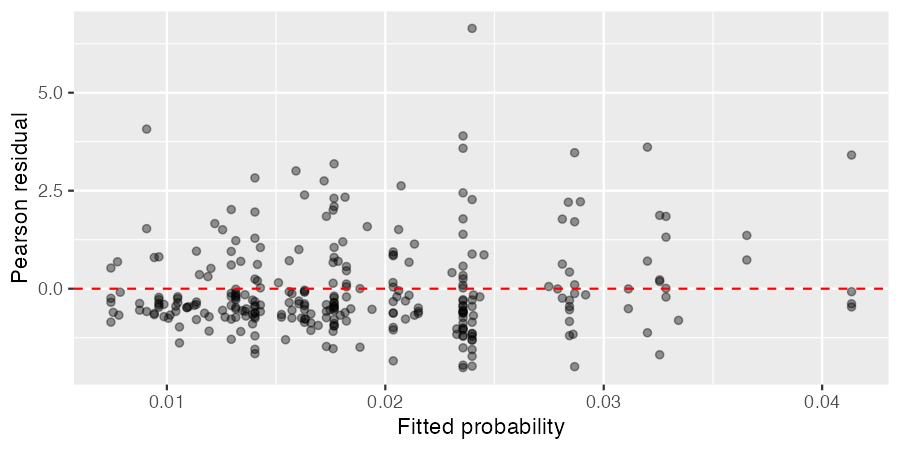
Most residuals are close to zero with no obvious trend, indicating the model captures the overall structure of the data well. One facility shows a relatively large residual and is more influential than the others, while the remaining residuals are spread along the fitted values as expected given the hierarchical partial pooling.

Model summary¶

The results of the fitted model are shown below. For brevity, the county random effects are not shown.


Iterations = 11001:111000
Thinning interval = 1 
Number of chains = 3 
Sample size per chain = 1e+05 

1. Empirical mean and standard deviation for each variable,
   plus standard error of the mean:

         Mean     SD  Naive SE Time-series SE
b[1]   0.2989 0.2348 0.0004287      0.0036989
b[2]   0.6113 0.2254 0.0004115      0.0038306
b[3]   0.5934 0.2125 0.0003880      0.0038373
mu    -4.4482 0.2171 0.0003965      0.0036734
sigma  0.4633 0.1023 0.0001868      0.0006561

2. Quantiles for each variable:

         2.5%     25%     50%     75%   97.5%
b[1]  -0.1530  0.1396  0.2956  0.4551  0.7683
b[2]   0.1822  0.4574  0.6076  0.7601  1.0669
b[3]   0.1898  0.4481  0.5894  0.7336  1.0252
mu    -4.8906 -4.5907 -4.4429 -4.2995 -4.0391
sigma  0.2912  0.3911  0.4533  0.5244  0.6922

Compared with the reference group (Community, <125 Beds), all three facility types have higher estimated probabilities of infection. On the log-odds scale, the posterior means are 0.30, 0.61, and 0.59 for Community 125–250 Beds, Community >250 Beds, and Major Teaching facilities, respectively. The 95% credible intervals for all three groups lie mostly above zero, suggesting that each facility type is likely associated with higher infection probability than the reference.

The overall county-level intercept has a posterior mean of –4.45, reflecting the baseline log-odds for the reference facility type, while the posterior standard deviation of the county-level random effects, $\sigma \approx$ 0.46, indicates moderate variation in baseline risk across counties.

Summary¶

The hierarchical Bayesian model provides partially pooled estimates of SSI risk for each facility while accounting for county-level variation. The posterior means indicate that all three non-reference facility types have higher log-odds of infection than the reference group, with 95% credible intervals largely above zero. The county-level standard deviation, σ ≈ 0.46, reflects moderate variation in baseline risk across counties. Compared with simpler models, the hierarchical approach stabilizes estimates for smaller facilities and better captures multilevel structure, offering a principled framework for facility-level risk estimation.

These results provide an initial view of facility- and county-level effects; a more formal comparison across models, along with further diagnostics and residual analysis, can be conducted in a future review. For now, this establishes a foundation for interpreting partial pooling and posterior uncertainty in SSI risk estimates.

References¶

Gelman, A., Carlin, J. B., Stern, H. S., Dunson, D. B., Vehtari, A., & Rubin, D. B. (2013). Bayesian Data Analysis (3rd ed.). Chapman. 10.1201/b16018